Simultaneous equations
In mathematics, simultaneous equations are a set of equations containing multiple variables. This set is often referred to as a system of equations. A solution to a system of equations is a particular specification of the values of all variables that simultaneously satisfies all of the equations. To find a solution, the solver needs to use the provided equations to find the exact value of each variable. Generally, the solver uses either a graphical method, the matrix method, the substitution method, or the elimination method. Some textbooks refer to the elimination method as the addition method, since it involves adding equations (or constant multiples of the said equations) to one another, as detailed later in this article.
This is a set of linear equations, also known as a linear system of equations:
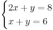
Solving this involves subtracting x + y = 6 from 2x + y = 8 (using the elimination method) to remove the y-variable, then simplifying the resulting equation to find the value of x, then substituting the x-value into either equation to find y.
The solution of this system is:

which can also be written as an ordered pair (2, 4), representing on a graph the coordinates of the point of intersection of the two lines represented by the equations.
Contents |
Finding solutions
Sometimes not all variables can be solved for, and so an answer for at least one variable must be expressed in terms of other variables and so the set of all solutions is infinite; this is typical for the case where the system has fewer equations than variables. If the number of equations is the same as the number of variables, then probably (but not necessarily) the system is exactly solvable in the sense that the set of its solutions is finite; for a system of linear equations in this case there is exactly one solution, for other systems to have several solutions is also typical. A consistent system is a system of equations with at least one solution. Sometimes a system is inconsistent, or has no solution;[1] this is typical for the case where the system has more equations than variables. If these rules about connection between number of solutions and numbers of equations and variables do not hold, then such situation is often referred to as dependence between equations or between their left parts. For instance, this occurs in linear systems if one equation is a simple multiple of the other (representing the same line, e.g. 2x + y = 3 and 4x + 2y = 6) or if the ratio of like variables in two linear equations is the same (representing parallel lines, e.g. 2x + y = 3 and 6x + 3y = 7 where the ratio of comparable letters is 3).
Systems of two equations in two real-value unknowns usually appear as one of five different types, having a relationship to the number of solutions:
- Systems that represent intersecting sets of points such as lines and curves, and that are not of one of the types below. This can be considered the normal type, the others being exceptional in some respect. These systems usually have a finite number of solutions, each formed by the coordinates of one point of intersection.
- Systems that simplify down to false (for example, equations such as 1 = 0). Such systems have no points of intersection and no solutions. This type is found, for example, when the equations represent parallel lines.
- Systems in which both equations simplify down to an identity (for example, x = 2x − x and 0y = 0). Any assignment of values to the unknown variables satisfies the equations. Thus, there are an infinite number of solutions: all points of the plane.
- Systems in which the two equations represent the same set of points: they are mathematically equivalent (one equation can typically be transformed into the other through algebraic manipulation). Such systems represent completely overlapping lines, or curves, etc. One of the two equations is redundant and can be discarded. Each point of the set of points corresponds to a solution. Usually, this means there are an infinite number of solutions.
- Systems in which one (and only one) of the two equations simplifies down to an identity. It is therefore redundant, and can be discarded, as per the previous type. Each point of the set of points represented by the other equation is a solution of which there are then usually an infinite number.
The equation x2 + y2 = 0 can be thought of as the equation of a circle whose radius has shrunk to zero, and so it represents a single point: (x = 0, y = 0), unlike a normal circle containing an infinity of points. This and similar examples show the reason why the last two types described above need the qualification "usually". An example of a system of equations of the first type described above with an infinite number of solutions is given by x = |x|, y = |y| (where the notation |•| denotes the absolute value function), whose solutions form a quadrant of the x-y plane. Another example is x = |y|, y = |x|, whose solution represents a ray. Another example is (x+1)(x+y)=0, (y+1)(x+y)=0, whose solution represents a line and a point.
Substitution method
Systems of simultaneous equations can be hard to solve unless a systematic approach is used. A common technique is the substitution method: Find an equation that can be written with a single variable as the subject, in which the left-hand side variable does not occur in the right-hand side expression. Next, substitute that expression where that variable appears in the other equations, thereby obtaining a smaller system with fewer variables. After that smaller system has been solved (whether by further application of the substitution method or by other methods), substitute the solutions found for the variables in the above right-hand side expression.
In this set of equations
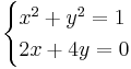
x is made the subject of the second equation:

then, this result is substituted into the first equation:
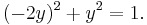
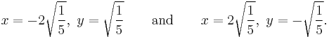
After simplification, this yields the solutions

and by substituting this in x = −2y the corresponding x values are obtained. The two solutions of the system of equations are then:
Elimination method
Elimination by judicious multiplication is the other commonly used method to solve simultaneous linear equations. It uses the general principles that each side of an equation still equals the other when both sides are multiplied (or divided) by the same quantity, or when the same quantity is added (or subtracted) from both sides. As the equations grow simpler through the elimination of some variables, a variable will eventually appear in fully solvable form, and this value can then be "back-substituted" into previously derived equations by plugging this value in for the variable. Typically, each "back-substitution" can then allow another variable in the system to be solved.
Matrices
Systems of equations may also be represented in terms of matrices, allowing various principles of matrix operations to be handily applied to the problem. Systems of simultaneous linear equations are studied in linear algebra; they are solved using Gaussian elimination or the Cholesky decomposition. To determine approximate solutions to general systems numerically on a computer, the n-dimensional Newton's method may be used. Algebraic geometry is essentially the theory of simultaneous polynomial equations. The question of effective computation with such equations belongs to elimination theory. See also Cramer's Rule, which computes the quotient of 2 determinants to calculate the solution.
Simultaneous equation models are a form of statistical model in the form of a set of linear simultaneous equations. They are often used in econometrics.
In modular arithmetic, simple systems of simultaneous congruences can be solved by the method of successive substitution.
Simultaneous equations are easier to solve using this method.
Least-squares
A set of linear simultaneous equations can be written in matrix form as Ax = y. If there are more equations than variables, the system is called overdetermined, and has (in general) no solutions. The system can then be changed to (ATA)x = ATy. The new system has as many equations as variables (the matrix ATA is a square matrix) and can be solved in the usual way. The solution is a least-squares solution of the original, overdetermined system, minimizing the Euclidean norm ||Ax − y||, a measure of the discrepancy between the two sides in the original system.
See also
References
- ^ Simmons, Bruce. "Mathwords". http://www.mathwords.com/i/inconsistent_system_of_equations.htm. Retrieved 11 October 2011.
External links
- Simultaneous equations
- Simultaneous linear equations solver
- Simultaneous Equation Solver Also computes the determinant, inverse, and LU Decomposition of the [A] Matrix.